Intro to Gaussian Processes: A Toy Model
When I started learning about Gaussian Processes (GPs), an endeavor that is still in progress, I came across various definitions, some of which I found a bit intuitive:
“A Gaussian process model describes a probability distribution over possible functions that fit a set of points.”
(Wang, Jie. An intuitive tutorial to Gaussian process regression.)
and others less so:
“A Gaussian process is a collection of random variables, any finite number of which have a joint Gaussian distribution.”
(Williams, Christopher KI, and Carl Edward Rasmussen. Gaussian processes for machine learning.)
(though I realized that less intuitive did not mean less important.) Gaussian Processes are a powerful modeling tool, and what helped me the most was seeing a GP in practice. In this post, I’ll walk through a simple toy example using the tinygp library . You can find the notebook I used for all the figures here.
Motivation: Why use a Gaussian Process?
Suppose you’ve collected a set of observations—maybe the daily temperature, stock prices, or (in my case) a measure of how stellar surfaces vary over time. For this example, let’s stick with temperature over time.
Imagine you’ve collected a few discrete observations. Maybe you now want to predict tomorrow’s temperature. Or maybe there’s a day in the past with missing data, and you want to estimate the temperature for that day.
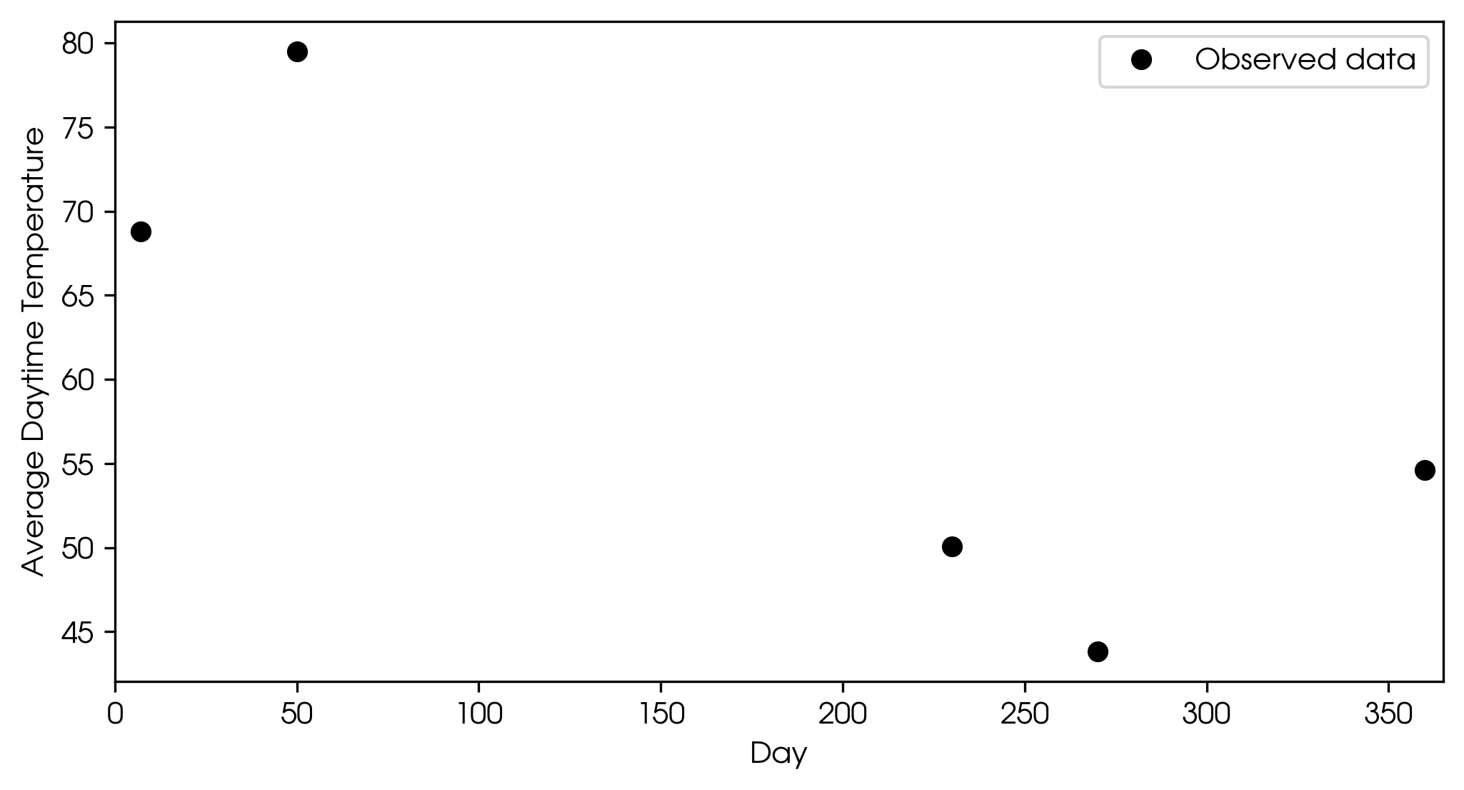 Example discrete observed temperatures over time.
This is a classic regression problem: given observed data, how can you predict values for new inputs?
How Gaussian Processes Help
GPs allow you to model relationships between your inputs (like days) and outputs (like temperature) without having to choose a specific functional form. Unlike fitting a straight line or a polynomial to your data (where you pre-choose a formula), GPs don't require you to make that choice beforehand. They are different in that (returning to the first definition), “GPs infer a distribution over possible functions that could explain the data, capturing both predictions and uncertainty.”
A key feature of GPs is that they don’t just output a single prediction. They also provide an uncertainty estimate, so you know how confident you are about each prediction. There’s a big difference between predicting that tomorrow’s temperature will be 70° ± 5°, or 70° ± 50°.
A Toy Model: GPs to Predict Temperature
Now let’s run a GP regression on the simulated temperature data. I used the Squared Exponential kernel, which I will discuss later, but these kernels essentially determine how smooth or wiggly the predicted function is. Let's take a look at the GP's prediction.
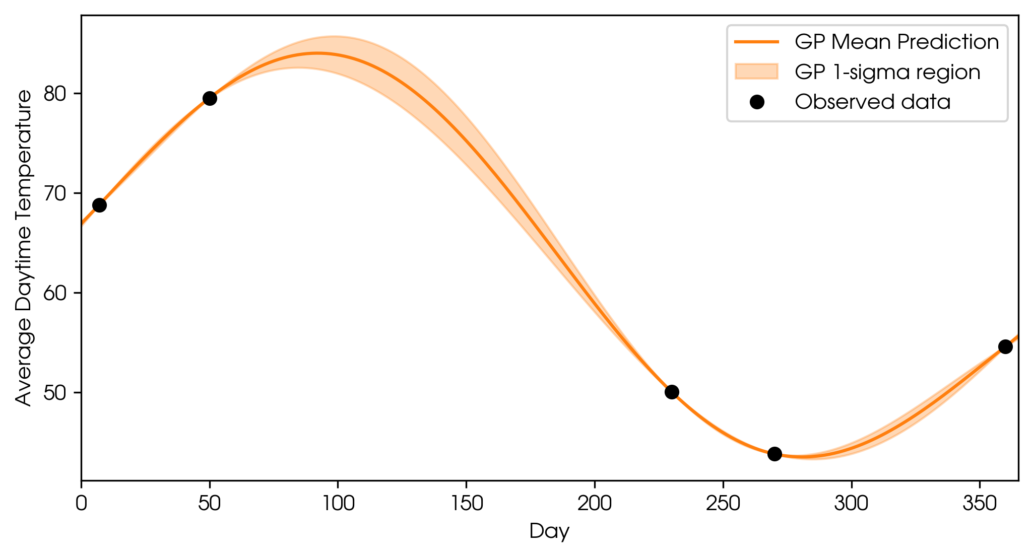 GP fit with no measurement error.
At the observed points, the GP prediction matches the data with zero uncertainty. This is assuming we measured the temperature perfectly. As you move further away from the observations, the uncertainty (shaded region) increases. If observations are made very close together, there is less uncertainty between them. But in real life, measurement error exists, so let’s add in some error bars to the observations and update the GP fit.
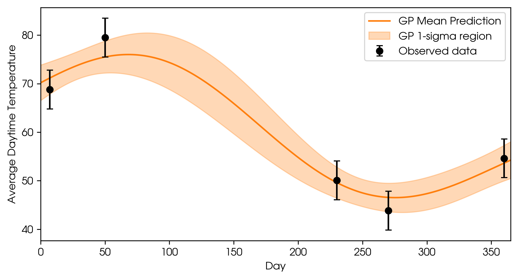 GP fit incorporating observational uncertainties.
That looks a bit more realistic.
The fitted GP now lets us interpolate (estimate between known data) or extrapolate (predict beyond the data range), and crucially, it tells us how much we can trust each prediction. For example, the temperature on day 100 is predicted to be 74.3° ± 5.6°. If you predict far beyond the last observation, uncertainty increases, reflecting our lack of information.
And that’s an example of how GPs can be used in regression: Given noisy, sparse data, GPs flexibly fit and quantify uncertainty for any input.
How does this all actually work?
Let’s revisit the second GP definition:
“A Gaussian process is a collection of random variables, any finite number of which have a joint Gaussian distribution.”
A random variable is simply a quantity whose outcome is uncertain, like the result of a dice roll. Let’s see how this relates to our GP: We can take a slice through the GP at day 100 and just look at the spread of predicted temperatures for that day.
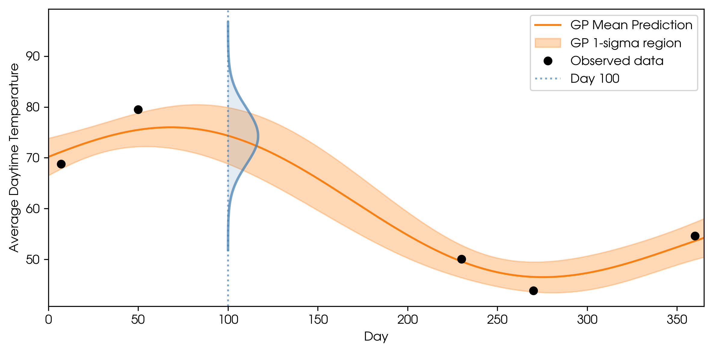 GP prediction for a single day (marginal).
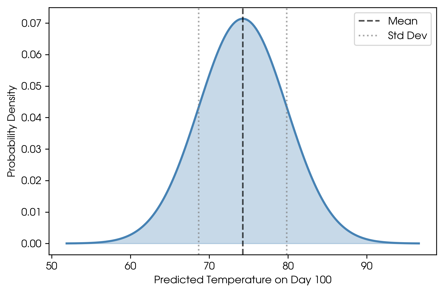 Marginal distribution for temperature on day 100.
This is the classic bell curve. It describes our single random variable (the temperature on day 100), and it is described by two values: a mean and standard deviation. The mean tells you the most likely value, and the standard deviation tells you the uncertainty on that value.
We can also take two slices—one at day 100 and one at day 150—and now we have two marginal distributions, each defined by its own mean and standard deviation. Now we’re looking at two random variables: the temperature on day 100 and the temperature on day 150.
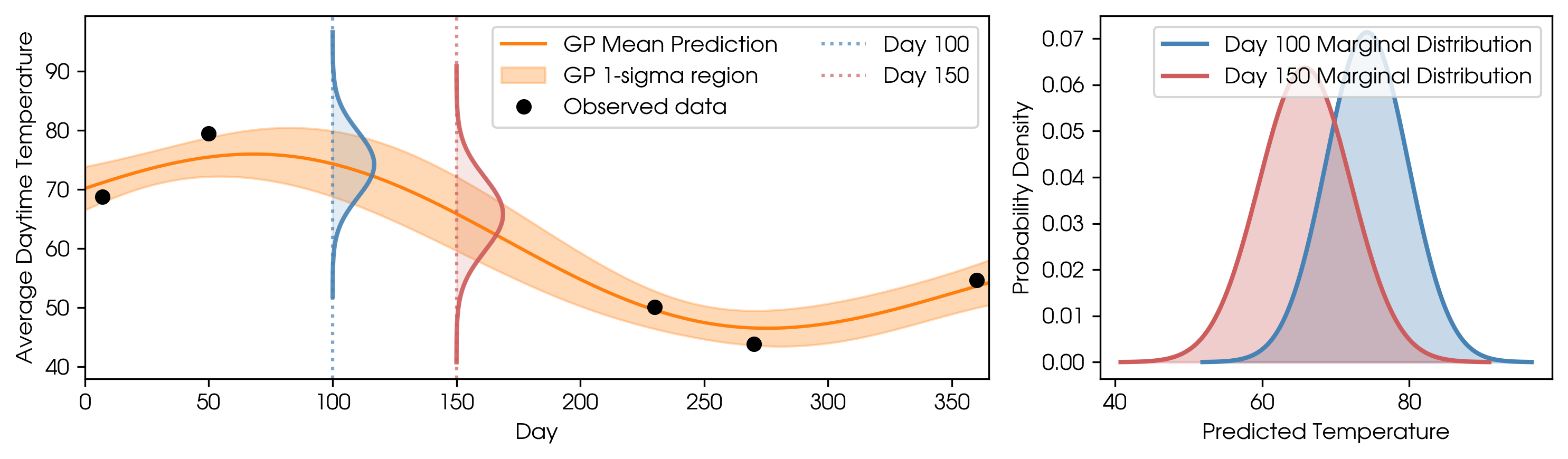 Two marginal distributions: temperatures on day 100 and day 150.
We can easily extend this to every single point, and now we have a collection of random variables: the temperature of any given day. The GP is simply “a collection of [these] random variables.”
Now onto the second part of the definition:
“…any finite number of which have a joint Gaussian distribution.”
If we plot the predicted temperatures for day 100 and day 150 as a joint distribution, we get a 2D Gaussian:
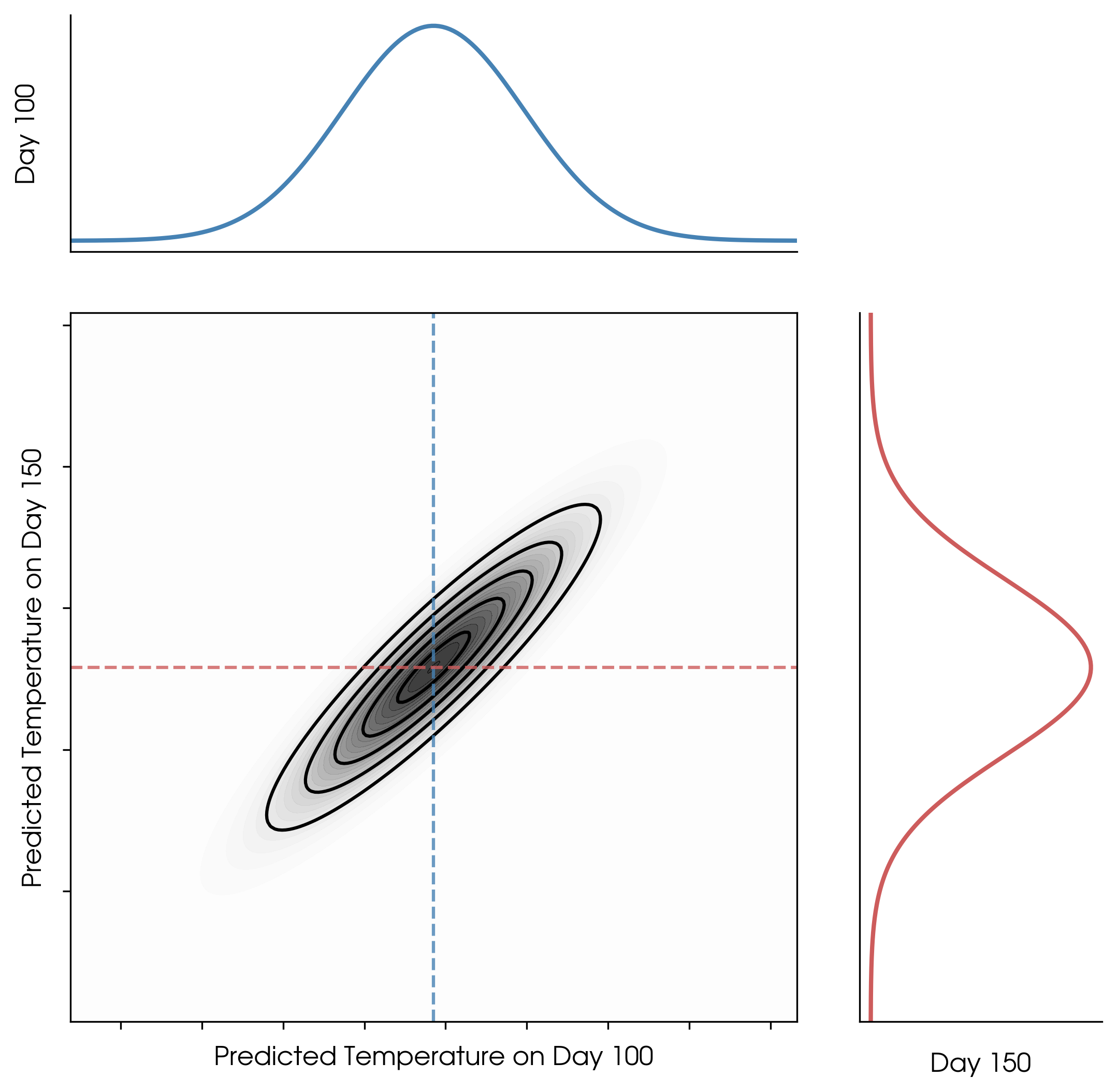 Joint distribution: pair of GP predictions (days 100 and 150).
This extends to higher dimensions too: any finite set of random variables in a GP is jointly Gaussian. In other words, a GP is an infinite-dimensional generalization of a Gaussian distribution. Every possible input is a random variable, and sets of those random variables are jointly Gaussian.
Components of a GP
While a single Gaussian distribution is defined by a mean and standard deviation, a GP is now defined by a mean function and a covariance matrix. Going from a mean value to a mean function is fairly straightforward: rather than a single predicted value for a single input value, the mean function now has a predicted value for every single possible input value. It essentially tells the GP what to fit around. For the weather example, I set the mean to be the average observed temperature.
The covariance matrix is slightly more complicated than just a simple extension of the standard deviation. Not only does each point have its uncertainty, but each pair of points has a quantified correlation—how much knowing one helps predict the other. For instance, in the weather example, the temperature on day 3 is likely to be similar to day 4 (highly correlated), but not necessarily similar to day 100 (weakly correlated). The covariance matrix captures the correlations between data points.
Choosing the right GP kernel
The GP kernel governs these correlations. It encodes your assumptions about how the data should behave: how correlated points should be, how smooth or wiggly the function might be, and whether there are underlying patterns like seasonality.
For the weather example, I used a squared exponential (SE) kernel. This kernel basically says: inputs closer together are more highly correlated (nearby temperatures should be similar), and the changes should happen smoothly (temperatures shouldn’t instantaneously spike or drop).
There are many kernels to choose from, each modeling different behaviors. Here are examples of four different kernels that I used to model the same weather data.
- Squared Exponential: Assumes outputs are similar for nearby inputs; favors smooth, gradual changes.
- Matern 3/2: Allows for less smoothness (more roughness) in the fitted curve.
- Exponential Sine Squared: Models repeating, periodic patterns.
- Squared Exponential + Exponential Sine Squared (Composite): Combines smooth trends with periodic/seasonal patterns. It is possible to combine any of the kernels to capture complex structure.
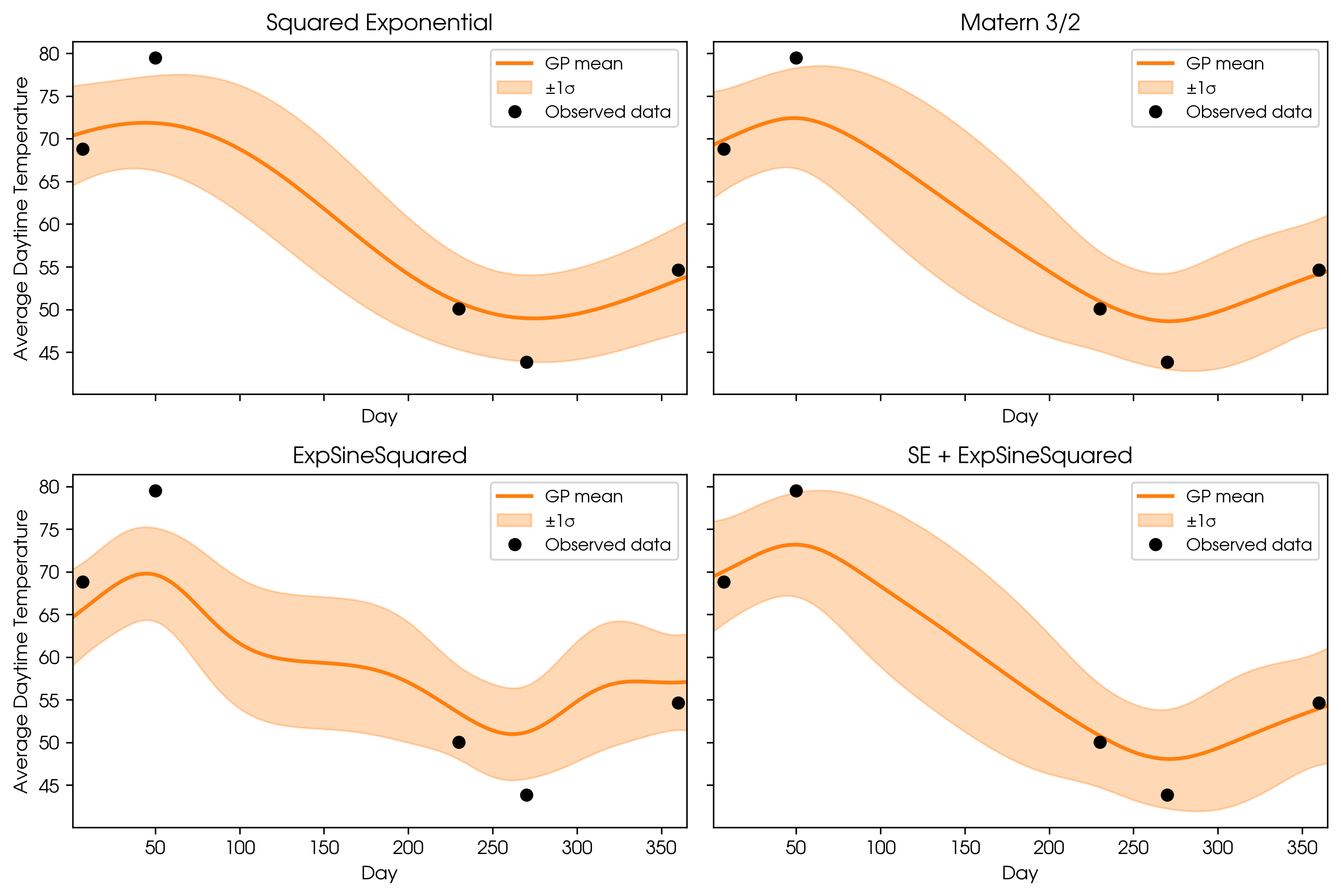 GP predictions using different kernels.
In summary, the kernel choice is crucial, as it tells the GP what kind of structure to expect in the data.
Kernel Hyperparameters: Amplitude & Length Scale
Once you’ve chosen your kernel, you need to set its hyperparameters:
- Amplitude: Controls how much the function can vary vertically. Larger amplitude means the GP expects bigger changes.
- Length scale: Controls how quickly the function can change. Small length scales let the GP fit rapid changes; large length scales create smoother functions.
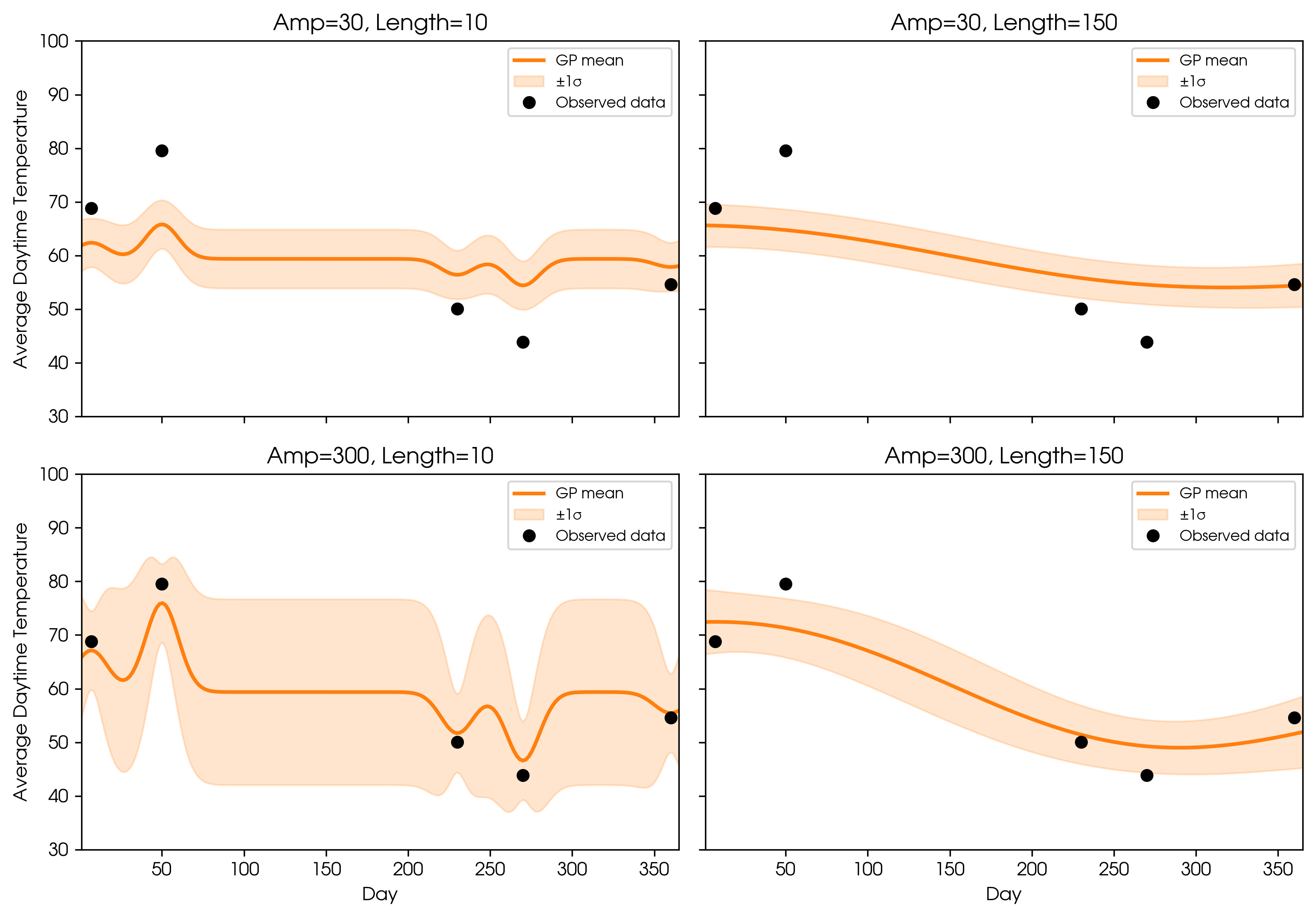 GP fits (squared exponential kernel) with different amplitudes and length scales.
Typically, these hyperparameters are fit to the data to avoid underfitting or overfitting, using techniques like maximizing marginal likelihood or Bayesian model comparison (through metrics like Bayesian Evidence).
Conclusion
Gaussian Processes are powerful tools for modeling and prediction amid noisy, limited, or complex data. They flexibly fit functions without needing a rigid formula and assign uncertainties to every prediction. However, it is crucial to carefully choose kernels and tune hyperparameters, which imparts assumptions about the phenomena being modeled. GPs enable robust predictions while communicating the confidence behind every result—a critical advantage in data-driven decision making.